TCR and CO2 concentration in AR6 and CMIP6
Doug McNeall
2023-01-06
We fit distributions to assessed quantiles of TCR in the literature, and then push those through the transfer function from Betts & McNeall (2018) to find an implied CO2 concentrayion at warming levels 1.5 and 2 degrees above preindustrial.
Quantiles from the literature
There are a number of sources of assessed probability distributions for TCR (sometimes just quantiles) in the literature. A complicating factor is that they often give a small number of different quantiles, or probability ranges, leaving a large number of potential distributions that would fit. For example, they might state a 66% probability range, without specifying the quantiles this range aplies to.
AR5 (assessed range)
“likley” range (66% probability)
1 - 2.5 deg C
Also “positive” and “extremely unlikely” (5% probability) above 3"
I interpret this as
| quantile | 0% | 17% | 83% | 97.5% |
|---|---|---|---|---|
| tcr | 0 | 1 | 2.5 | 3 |
But it’s possible to interpret that upper quantile as 95%, as there is ambiguity around whether the 5% probability should be split over both tails of the distribution. . I’ll update this possible inconsistancy as I find out.
CMIP5 models
AR5 Box 12.2 states:
“5 to 95% range of CMIP5 (1.2°C to 2.4°C; see Table 9.5), is positive and extremely unlikely greater than 3°C.” As this explicitly mentions the 95% and the “extremely unlikely” statement, that lends evidence that “extremely unlikely” is spread over both tails, and refers to the 97.5th percentile.
| quantile | 0% | 5% | 95% | 97.5% |
|---|---|---|---|---|
| tcr | 0 | 1.2 | 2.5 | 3 |
Schurer eta al (2018)
Multimodel mean with increased variance for model uncertainty
| quantile | 5% | 50% | 95% |
|---|---|---|---|
| tcr | 1.2 | 1.7 | 2.4 |
Sherwood et al (2020)
Likely (66% probability) range
| quantile | 16% | 50% | 84% |
|---|---|---|---|
| tcr | 1.5 | 1.8 | 2.2 |
Jiménez-de-la Cuesta and Mauritsen (2019)
| quantile | 5% | 50% | 95% |
|---|---|---|---|
| tcr | 1.17 | 1.7 | 2.16 |
Tokarska et al (2020)
| quantile | 16% | 50% | 84% |
|---|---|---|---|
| tcr | 1.2 | 1.6 | 2.0 |
Njisse et al. (2020)
Njisse et al. (2020) CMIP5 models
| quantile | 5% | 16% | 50% | 84% | 95% |
|---|---|---|---|---|---|
| tcr | 1.1 | 1.4 | 1.7 | 2.1 | 2.4 |
Njisse et al. (2020) CMIP6 models
| quantile | 5% | 16% | 50% | 84% | 95% |
|---|---|---|---|---|---|
| tcr | 1 | 1.29 | 1.68 | 2.05 | 2.3 |
Distributions used in Betts & McNeall (2018)
## [1] 1.302494 2.197506## [1] 1.004157 2.495843Other distributions to might fit TCR better
The distribution from Richardson is asymmetric, and there is evidence that the other distributions representing scientists beliefs are asymmetric too. Normal distributions can easily place significant probability below zero, which is explicitly ruled out in the AR5 assessment.
Other distributions, such as Gamma or lognormal, might fit better.
For example, here is a Gamma distribution with some sensible-looking parameters.

Fit distributions to the Richardson samples from their TCR distribution
Fit the Gamma distribution, starting from the above parameters.
Fit a lognormal distribution to Richardson
This seems to fit a little better than the Gamma distribution.
Fit a lognormal distribution to all of the distributions from the literature
## The fitting procedure 'L-BFGS-B' was successful!## $par
## [1] 0.4370346 0.4324224
##
## $value
## [1] 0.0002381779
##
## $counts
## function gradient
## 13 13
##
## $convergence
## [1] 0
##
## $message
## [1] "CONVERGENCE: REL_REDUCTION_OF_F <= FACTR*EPSMCH"
## The fitting procedure 'L-BFGS-B' was successful!## $par
## [1] 0.5528290 0.2264219
##
## $value
## [1] 3.430531e-05
##
## $counts
## function gradient
## 9 9
##
## $convergence
## [1] 0
##
## $message
## [1] "CONVERGENCE: REL_REDUCTION_OF_F <= FACTR*EPSMCH"
## The fitting procedure 'L-BFGS-B' was successful!## $par
## [1] 0.5304240 0.2106881
##
## $value
## [1] 1.41057e-07
##
## $counts
## function gradient
## 12 12
##
## $convergence
## [1] 0
##
## $message
## [1] "CONVERGENCE: REL_REDUCTION_OF_F <= FACTR*EPSMCH"
## The fitting procedure 'L-BFGS-B' was successful!## $par
## [1] 0.5917034 0.1926020
##
## $value
## [1] 1.712434e-05
##
## $counts
## function gradient
## 20 20
##
## $convergence
## [1] 0
##
## $message
## [1] "CONVERGENCE: REL_REDUCTION_OF_F <= FACTR*EPSMCH"
## The fitting procedure 'L-BFGS-B' was successful!## $par
## [1] 0.5171894 0.3200099
##
## $value
## [1] 0.0001466232
##
## $counts
## function gradient
## 12 12
##
## $convergence
## [1] 0
##
## $message
## [1] "CONVERGENCE: REL_REDUCTION_OF_F <= FACTR*EPSMCH"
## The fitting procedure 'L-BFGS-B' was successful!## $par
## [1] 0.5333458 0.2088702
##
## $value
## [1] 4.883697e-05
##
## $counts
## function gradient
## 13 13
##
## $convergence
## [1] 0
##
## $message
## [1] "CONVERGENCE: REL_REDUCTION_OF_F <= FACTR*EPSMCH"
## The fitting procedure 'L-BFGS-B' was successful!## $par
## [1] 0.5011289 0.2300069
##
## $value
## [1] 0.0001314229
##
## $counts
## function gradient
## 13 13
##
## $convergence
## [1] 0
##
## $message
## [1] "CONVERGENCE: REL_REDUCTION_OF_F <= FACTR*EPSMCH"
## The fitting procedure 'L-BFGS-B' was successful!## $par
## [1] 0.5279935 0.1582696
##
## $value
## [1] 0.0002056946
##
## $counts
## function gradient
## 13 13
##
## $convergence
## [1] 0
##
## $message
## [1] "CONVERGENCE: REL_REDUCTION_OF_F <= FACTR*EPSMCH"
## The fitting procedure 'L-BFGS-B' was successful!## $par
## [1] 0.4561703 0.2572126
##
## $value
## [1] 0.0001190927
##
## $counts
## function gradient
## 13 13
##
## $convergence
## [1] 0
##
## $message
## [1] "CONVERGENCE: REL_REDUCTION_OF_F <= FACTR*EPSMCH"
Plot all of the lognormal fits

How close are the lognormal fits?
This section plots the fitted quantiles (on the y axis) against the given quantiles (from the literature, on the x axis). Lower quantiles (with values below 3) are in general well fitted. The fitted upper quantile of the distribution is much higher than suggested by the given distribution, suggesting that the fit assigns too much probability to the upper tail of the distribution than the assesed distribution would suggest is right.


## The fitting procedure 'L-BFGS-B' was successful!
## The fitting procedure 'L-BFGS-B' was successful!
## The fitting procedure 'L-BFGS-B' was successful!
## The fitting procedure 'L-BFGS-B' was successful!
## The fitting procedure 'L-BFGS-B' was successful!
## The fitting procedure 'L-BFGS-B' was successful!
## The fitting procedure 'L-BFGS-B' was successful!
## The fitting procedure 'L-BFGS-B' was successful!
## The fitting procedure 'L-BFGS-B' was successful!
## The fitting procedure 'L-BFGS-B' was successful!

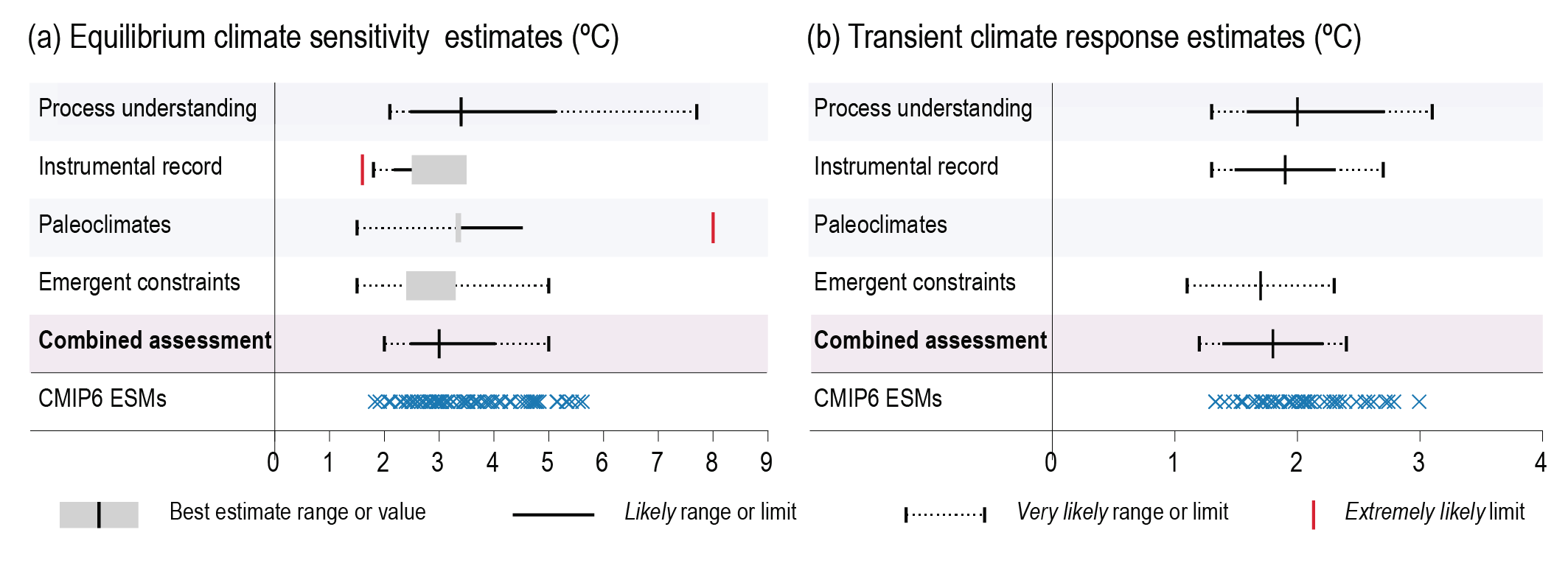
TCR in the AR6
Caption https://www.ipcc.ch/report/ar6/wg1/figures/chapter-7/figure-7-18
Big version (in the report) https://www.ipcc.ch/report/ar6/wg1/downloads/figures/IPCC_AR6_WGI_Figure_7_18.png
Somebody has calculated the CMIP6 TCR values! (this could be useful)
Plot TCR fitted lognormal distributions
Blue dots are CMIP6 model TCR measured and published in the AR6

Plot projected CO2 at warming levels
Transfer function
Sample from the lognormal distributions and push through the TCR transfer function
Truncated TCR values below 0.5, as you get odd things happening.
Also project CMIP6 TCR into CO2 concentration at GWLs by pushing the AR6-published TCR values through the transfer function.

Load CMIP6 models actual CO2 at 1.5 and 2 degrees at SSPs
This section plots the CO2 measured at warming levels 1.5, 2, 3 & 4 degrees in CMIP6 models against the CO2 levels you would expect from projecting their measured TCR through the transfer function.
Measured CO2 levels are consistently below what you would expect from their TCR.
SSP585
 SSP370

SSP245
